Synthesis of Bennett Mechanism (JupyterNTB Tutorial)

This Jupyter notebook serves as an example of using the package for mechanism synthesis. Run it live on Binder platform clicking on the following badge:

Link to the source notebook: https://github.com/hucik14/rational-linkages/blob/main/docs/source/tutorials/synthesis_bennett.ipynb

# in case of errors, make sure to have the latest version of the rational-linkages package installed (uncomment the following line and run the cell)
# !pip install --upgrade rational-linkages[opt]

# you can ignore PyQt errors as this backend is not used for Jupyter Notebooks
# initial import of the required libraries
%matplotlib inline

from rational_linkages import (Plotter, MotionInterpolation, TransfMatrix, RationalMechanism)

Poses definition

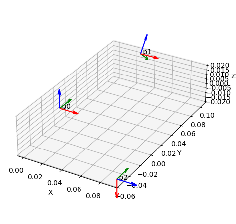
Bennett mechanism can be synthesised from a quadratic motion curve. This curve can be obtained from interpolation of 3 given poses. Poses can be defined as transformation matrices or dual quaternions. This examples creates poses from roll, pitch, yaw angles and desired translations.

Pose p0 is set to identity, which will yield the univariate rational function after the interpolation. It is always possible to perform transformation of the whole motion curve (including mechanism itself) to desired end-effector pose.

# for simplification, p0 is the identity matrix
p0 = TransfMatrix()

p1 = TransfMatrix.from_rpy_xyz([-40, 0, 0], [0.030, 0.1, 0.02], unit='deg')
p2 = TransfMatrix.from_rpy_xyz([0, 90, 0], [0.09, -0.05, -0.02], unit='deg')

poses = [p0, p1, p2]  # list of the transformation matrices

for i, pose in enumerate(poses):
    print(f'Pose {i}:')
    print(pose)

Pose 0:
[[1., 0., 0., 0.],
 [0., 1., 0., 0.],
 [0., 0., 1., 0.],
 [0., 0., 0., 1.]]
Pose 1:
[[ 1.          ,  0.          ,  0.          ,  0.          ],
 [ 0.03        ,  1.          ,  0.          ,  0.          ],
 [ 0.1         ,  0.          ,  0.7660444431,  0.6427876097],
 [ 0.02        ,  0.          , -0.6427876097,  0.7660444431]]
Pose 2:
[[ 1.  ,  0.  ,  0.  ,  0.  ],
 [ 0.09,  0.  ,  0.  ,  1.  ],
 [-0.05,  0.  ,  1.  ,  0.  ],
 [-0.02, -1.  ,  0.  ,  0.  ]]

You can notice that the matrices follow “european” convetion, i.e. the first row are homogeneous coordinates, the first column is the translation vector, and rotation matrix is in the second to last column/row.

We chose p2 to be identity matrix, which returns monomial curve. This means, that the curve will interpolate exactly the desired poses. This pose can be arbitrary, but since the factorization produces later monomial polynoms, the whole mechanism will undergo static transformation by p2.

# initiate plotter
myplt = Plotter(jupyter_notebook=True, arrows_length=0.02)
for i, pose in enumerate(poses):
    myplt.plot(pose, label=f'p{i}')

Poses interpolation

# obtain curve from poses
curve = MotionInterpolation.interpolate(poses)

print('')
print('Interpolated curve:')
print(curve)

myplt = Plotter(jupyter_notebook=True, arrows_length=0.02, steps=300)
for i, pose in enumerate(poses):
    myplt.plot(pose, label=f'p{i}')
myplt.plot(curve, interval='closed')

Interpolated curve:
RationalCurve([2.573049098872*t**2 - 1.68788693606722*t + 0.247312168627015, -0.412186947711691*t, 0.247312168627015 - 0.247312168627015*t, 0, -0.00618280421567536, -0.00338494569699111*t - 0.0136021692744858, 0.00618280421567536 - 0.0586846513101482*t, -0.023278164797957*t - 0.00865592590194551])

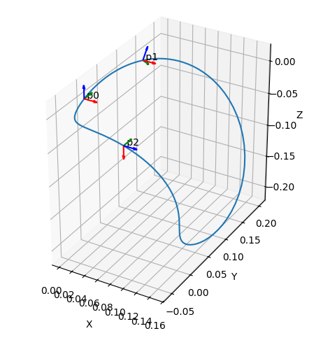
Keep in mind, that the curve above is 8-dimensional curve that interpolates both, position and orientation. The plotted blue curve shows only position.

Motion factorization

Synthesize mechanism that can follow given motion curve

mechanism = RationalMechanism(curve.factorize())

myplt = Plotter(mechanism=mechanism, jupyter_notebook=True, arrows_length=0.02, steps=300)
for i, pose in enumerate(poses):
    myplt.plot(pose, label=f'p{i}')

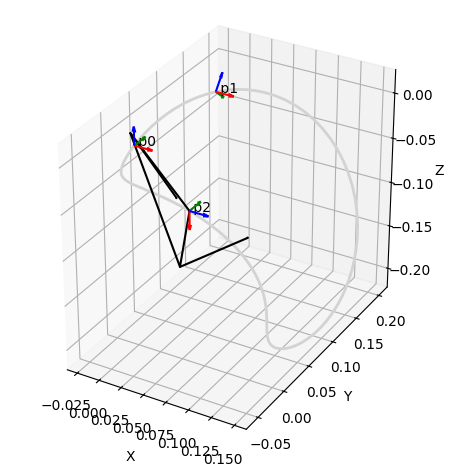
On the figure above, a Bennett mechanism (black) that can achieve with its tool frame (tool link is represented with purple dashed lines) is shown. This only very simple line model with collisions, which can be checked using following line.

mechanism.collision_check()

Collision check started...
--- number of tasks to solve: 20 ---
--- collision check finished in 0.27808713912963867 seconds.
No collisions found.

Collision-free design

It is possible to run collision-free linkage using the combinatorial search algorithm. Since it is a time demanding task, the following line is commented.

# mechanism.collision_free_optimization(max_iters=10)

A solution was already calculated before for following shifts of combinations. Lists of combinations can be also inserted in to the search, the same as starting iteration, etc. Please, read more carefully the tutorial documentation page on this topic.

comb_links = [(0, 0, 0, -1)]
comb_joints = [(-1, 1, 1, -1, 1, -1, -1, 1)]
mechanism.collision_free_optimization(min_joint_segment_length=0.003,
                                       combinations_links=comb_links,
                                       combinations_joints=comb_joints)

Starting combinatorial search algorithm...
--- iteration: 1, shift_value: 0.012022695085620426, sequence 1 of 1: (0, 0, 0, -1)
Collision check started...
--- number of tasks to solve: 2 ---
--- collision check finished in 0.1417539119720459 seconds.
No collisions found.

Collision-free solution for links found, starting joint search...
--- joint search. Shift_value: 0.0015, sequence 1 of 1: (-1, 1, 1, -1, 1, -1, -1, 1)
Collision check started...
--- number of tasks to solve: 20 ---
--- collision check finished in 0.25880980491638184 seconds.
No collisions found.
Search was successful, collision-free solution found.

[[np.float64(-0.0015), np.float64(0.0015)],
 [np.float64(0.0015), np.float64(-0.0015)],
 [np.float64(0.0015), np.float64(-0.0015)],
 [np.float64(-0.013522695085620425), np.float64(-0.010522695085620426)]]

The animated mechanism can be seen on the GIF bellow.

Generation of physical parameters

The following line can obtains Denavit-Hartenberg parameters and joint connection parameters for pre-prepared CAD models. The scale=1000 argument scales the length by 1000 units to change from meters to millimeters.

design_parameters = mechanism.get_design(scale=1000, unit='deg')

Denavit-Hartenberg parameters and connection points parameters:
---
Link 0: d = 0.000000000000, a = 68.274374144472, alpha = 128.164082452496
cp_0 = -0.003930034765, cp_1 = -0.012675053357
---
Link 1: d = 0.000000000000, a = 82.009314425718, alpha = 109.193213394822
cp_0 = -0.033675053357, cp_1 = -0.123707190060
---
Link 2: d = -0.000000000000, a = 68.274374144472, alpha = 128.164082452496
cp_0 = -0.102707190060, cp_1 = 0.018406607253
---
Link 3: d = -0.000000000000, a = 82.009314425718, alpha = 109.193213394822
cp_0 = -0.002593392747, cp_1 = -0.024930034765
======
Points which define the joint axes of mechanism in the world frame, at home configuration. Note that joint0 and jointN are part of the base_link joints:
Joint 0:
    pt0 = [26.263172980572, 24.882073222352, -70.406432037080],
    pt1 = [22.758825204109, 43.763613027380, -61.908961751594]
Joint 1:
    pt0 = [-3.782879537964, 76.949490357191, -117.526303731011],
    pt1 = [-21.818589885550, 84.657411841013, -110.022897927165]
Joint 2:
    pt0 = [68.540471224932, -3.575366597281, -10.261651024297],
    pt1 = [65.036123448469, 15.306173207748, -18.759121309782]
Joint 3:
    pt0 = [78.705386485712, 75.896326250587, -115.478390646948],
    pt1 = [60.669676138125, 83.604247734409, -122.981796450794]

To model a linkage of your own, generate CAD STEP model using one of the methods on this site: https://rational-linkages.readthedocs.io/latest/tutorials/cad.html