Plotting Examples
The package class Plotter provides a simple interface to plotting rational
mechanisms, and related objects like curves, poses, lines, points, etc.
The Plotter returns either PlotterPyqtgraph or PlotterMatplotlib, as both backends
are supported and share most of the functionality. The default backend is PlotterPyqtgraph, which is
faster and therefore more suitable for interactive plotting. The PlotterMatplotlib is more suitable for
publishing, as it provides better quality and cleanness (thanks to vector graphics) of the output images.
Static plotting
By default, the plots are not interactive. This is suitable for simple plots with static objects:
"""
# Plotting static objects
"""

from rational_linkages import Plotter, DualQuaternion, PointHomogeneous, NormalizedLine, TransfMatrix


# create plotter object, arg steps says how many discrete steps will be used for
# plotting curves
plt = Plotter(backend='matplotlib')

# create two DualQuaternion objects
identity = DualQuaternion()
pose1 = DualQuaternion([0, 0, 1, 0, 0, -0.5, 1, 0])
pose2 = TransfMatrix.from_rpy_xyz([0, -90, 0], [0, 0, 0.5], unit='deg')

# create a point with homogeneous coordinates w = 1, x = 2, y = -3, z = 1.5
point = PointHomogeneous([1, 2, -3, 1.5])

# create a normalized line from direction vector and the previously specified point
line = NormalizedLine.from_direction_and_point([0, 0, 1], point.normalized_euclidean())

# plot the objects
# 1-line command
plt.plot(identity, label='base')
plt.plot(point, label='pt')
plt.plot(line, label='l1')
# or for cycle
for i, obj in enumerate([pose1, pose2]):
    plt.plot(obj, label='p{}'.format(i + 1))

plt.show()
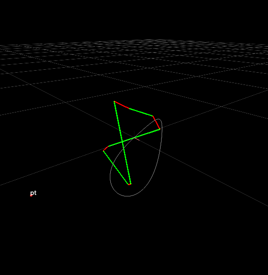
Which will result in the following image:

Additionally, it is also possible to plot motion curve of a mechanism.
from rational_linkages import Plotter
from rational_linkages.models import bennett_ark24


m = bennett_ark24()

p = Plotter(backend="matplotlib", arrows_length=0.03)
p.plot(m.curve(), interval='closed', with_poses=True)
p.show()
Which will result in the following image:

Interactive plotting
In the interactive mode, the mechanisms can be animated.
from rational_linkages import Plotter, PointHomogeneous
from rational_linkages.models import bennett_ark24


# load the mechanism
m = bennett_ark24()

# create an interactive plotter object
plt = Plotter(mechanism=m, arrows_length=0.05)

# create a point with homogeneous coordinates w = 1, x = 2, y = -3, z = 1.5
point = PointHomogeneous([1, 0.5, -0.75, 0.25])

plt.plot(point, label='pt')
plt.show()
Which will result in the following image. The interactive plotter can be used to animate the mechanism using the slider widget bellow the plot. The sliders on the left side of the plot can be used to change the design parameters of the mechanism.
If the argument backend='matplotlib' is used, the plot will switch to this mode:

Scaling of plotted objects
Sometimes, the mechanism is too large or too small to be plotted along with its
tool frame, or the range sliders that control physical realization have very high/low
limits. In such cases, it is possible to use key word arguments arrows_length and
joint_sliders_lim when initializing the plotter using Plotter class.
The joint_sliders_lim specifies the limits of the range sliders, and the arrows_length
to adjust the size of the length of the frames/poses that are plotted.
"""
# Interactive plotting with a loaded mechanism model, adjusted scaling
"""

from rational_linkages import Plotter
from rational_linkages.models import bennett_ark24 as bennett


m = bennett()

plt = Plotter(mechanism=m, arrows_length=0.05, joint_sliders_lim=0.5)
plt.show()
Optional tool frames
When an object RationalMechanism is plotted, an optional argument
show_tool=True can be used to plot its tool frame, as showed in the previous
examples.
However, the tool of a mechanism frame can be handled in three ways:
1. The tool frame is not specified, i.e.
None– then, the tool frame is attached by two connecting lines to the last link and follows the mechanism’s motion curve.2. The tool frame is specified as string tool=’mid_of_last_link’, which calculates and places the tool frame in the middle of the last link, with x-axis coinciding with the link.
3. The tool frame is specified as
DualQuaternionobject using argumenttool=DualQuaternion()– then, this tool frame is attached to the last link.
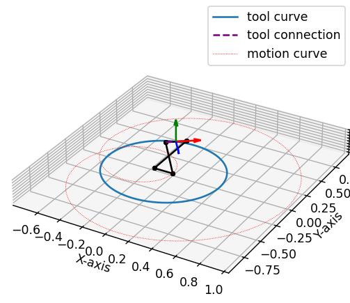
The following examples show the three options.
"""
# Tool frame on motion curve
"""

from rational_linkages import (RationalMechanism, DualQuaternion,
                               Plotter, MotionFactorization)


# Define factorizations
f1 = MotionFactorization([DualQuaternion([0, 0, 0, 1, 0, 0, 0, 0]),
                          DualQuaternion([0, 0, 0, 2, 0, 0, -1, 0])])

f2 = MotionFactorization([DualQuaternion([0, 0, 0, 2, 0, 0, -1 / 3, 0]),
                          DualQuaternion([0, 0, 0, 1, 0, 0, -2 / 3, 0])])

# Create mechanism
m = RationalMechanism([f1, f2])

# Create plotter
plt = Plotter(mechanism=m, backend='matplotlib', arrows_length=0.2)
plt.show()

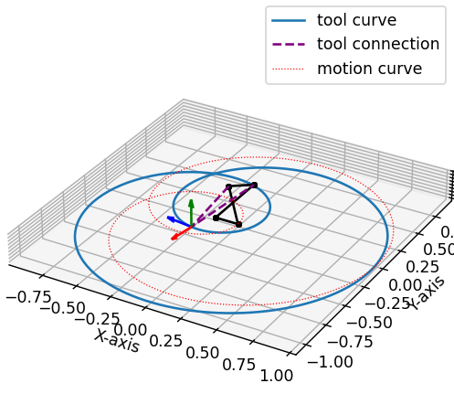
"""
# Tool frame in the middle of the last link
"""

from rational_linkages import (RationalMechanism, DualQuaternion,
                               Plotter, MotionFactorization)


# Define factorizations
f1 = MotionFactorization([DualQuaternion([0, 0, 0, 1, 0, 0, 0, 0]),
                          DualQuaternion([0, 0, 0, 2, 0, 0, -1, 0])])

f2 = MotionFactorization([DualQuaternion([0, 0, 0, 2, 0, 0, -1 / 3, 0]),
                          DualQuaternion([0, 0, 0, 1, 0, 0, -2 / 3, 0])])

# Create mechanism
m = RationalMechanism([f1, f2], tool='mid_of_last_link')

# Create plotter
plt = Plotter(mechanism=m, backend='matplotlib', arrows_length=0.2)

# Plot the default motion curve
plt.plot(m.get_motion_curve(), label='motion curve', interval='closed',
       color='red', linewidth='0.7', linestyle=':')
plt.show()
"""
# Tool frame specified as DualQuaternion
"""

from rational_linkages import (RationalMechanism, DualQuaternion, TransfMatrix,
                               Plotter, MotionFactorization)


# Define factorizations
f1 = MotionFactorization([DualQuaternion([0, 0, 0, 1, 0, 0, 0, 0]),
                          DualQuaternion([0, 0, 0, 2, 0, 0, -1, 0])])

f2 = MotionFactorization([DualQuaternion([0, 0, 0, 2, 0, 0, -1 / 3, 0]),
                          DualQuaternion([0, 0, 0, 1, 0, 0, -2 / 3, 0])])

# Create tool frame from transformation matrix
tool_matrix = TransfMatrix.from_rpy_xyz([90, 0, 45], [-0.2, 0.5, 0], unit='deg')
tool_dq = DualQuaternion(tool_matrix.matrix2dq())

# Create mechanism
m = RationalMechanism([f1, f2], tool=tool_dq)

# Create plotter
plt = Plotter(mechanism=m, backend='matplotlib', arrows_length=0.2)

# Plot the default motion curve
plt.plot(m.get_motion_curve(), label='motion curve', interval='closed',
       color='red', linewidth='0.7', linestyle=':')
plt.show()
Generating frames (for animation)
Both classes PlotterPyqtgraph and PlotterMatplotlib have various methods to generate a figure
or set of figures for animation purposes. See for more details the implementation:
PlotterMatplotlib.save_image(), PlotterMatplotlib.animate(), PlotterMatplotlib.animate_angles(),
InteractivePlotterWidget.on_save_figure_box() (use GUI), PlotterPyqtgraph.animate_rotation().