ARK 2024 Paper - Extended Information

IMPORTANT NOTE: there has been updates to Rational Linkages, therefore the values output of the method RationalMechanism.get_design() will differ. However, to keep consistency with the Onshape models shared bellow, the old values are kept here. To obtain mechanism design for your particular linkage, generate STEP model as shown in CAD Modeling tutorial.

This page contains the extended information for the paper submitted to conference ARK 2024, Lublijana, Slovenia, under the title: Rational Linkages: From Poses to 3D-printed Prototypes

Please, make sure to install the package before running the following examples, as described in the installation section.

Bennett mechanism example

A Bennett mechanism was synthesized by Brunnthaler et al.[1]. It performs the motion \(C(t)\) given byt the following equation

\[\begin{split}C(t) = \begin{bmatrix} 0 \\ 22134 + 39870 t + 4440 t^2 \\ -42966+9927t+16428 t^2 \\ -115878-73843t-37296 t^2 \\ 0 \\ -7812-14586t-1332 t^2 \\ 6510-1473t-2664 t^2 \\ -3906-1881t-1332 t^2 \\ \end{bmatrix}\end{split}\]

This equation serves as the input for the following script.

from rational_linkages import RationalCurve, RationalMechanism, FactorizationProvider, Plotter
import numpy as np

coeffs = np.array([[0, 0, 0],
                   [4440, 39870, 22134],
                   [16428, 9927, -42966],
                   [-37296, -73843, -115878],
                   [0, 0, 0],
                   [-1332, -14586, -7812],
                   [-2664, -1473, 6510],
                   [-1332, -1881, -3906]])

# define a rational curve object
c = RationalCurve.from_coeffs(coeffs)

# factorize the curve
factors = c.factorize()

# define a mechanism object
m = RationalMechanism(factors)

# define a plotter object, set interactive mode and number of discrete steps
# to plot the curve
p = Plotter(mechanism=m, steps=500, arrows_length=0.05)

# plot the mechanism
p.show()

The curve \(C(t)\) is of degree 2 in the variable \(t\), and can be factorized in the following form:

\[C(t) = (t - h_1)(t - h_2) = (t - k_1)(t - k_2)\]

The Dual Quaternions that relate to the revolute joints of the Bennett linkage were obtained using the FactorizationProvider class. The resulting Study parameters are:

\[\begin{split}h_1 = \begin{bmatrix} -1.38983921 \\ 0.68767732 \\ -0.71589104 \\ 0.70107044 \\ 0 \\ 0.279825759 \\ 0.233347361 \\ -0.03619970 \\ \end{bmatrix} h_2 = \begin{bmatrix} -0.45127753 \\ -1.18920251 \\ 0.02617346 \\ -1.06457999 \\ 0 \\ -0.205980947 \\ 0.0051919116 \\ 0.230221262 \\ \end{bmatrix} k_1 = \begin{bmatrix} -0.45127753 \\ -1.37336934 \\ -0.65524381 \\ 0.4824214 \\ 0 \\ -0.11647403 \\ 0.242442406 \\ -0.00228634 \\ \end{bmatrix} k_2 = \begin{bmatrix} -1.38983921 \\ 0.87184415 \\ -0.03447376 \\ -0.84593095 \\ 0 \\ 0.190318846 \\ -0.00390313 \\ 0.1963079 \\ \end{bmatrix}\end{split}\]

The resulting mechanism is plotted unsing the Plotter class. The resulting plot is shown in the figure below.

Physical modelling of Bennett mechanism

Since the default line model cannot be directly used for 3D printing, because the joint segments are too small. Therefore, the sliders on the left side of the plotter window can be used to control the placement of the physical conneting points on a joint-axis. An example is shown in Figure below.

When a user is satisfied with the placement of the connecting points, the mechanism can be saved to a file using the “Save with filename:” textbox, filling the filename and pressing Enter button on the keyboard. Eventually, it is possible to save the mechanism using the method RationalMechanism.save() in Python console. Then, the mechanism can be loaded and checked for collisions using the script below.

If there are no collisions, the output in the console will write “No collisions found.” If there are collisions, it will return list of parameter \(t\) values, where the collisions happen. This value can be passed to the plotting window at the textbox Set param t [-].

from rational_linkages.models import bennett_ark24

# on Windows, the script has to be run inside the if __name__ == '__main__'
# so the parallel processing can be used
if __name__ == '__main__':
    # load the mechanism
    m = bennett_ark24()

    # check for collisions
    m.collision_check(parallel=True)

    # generate the design
    dh, cp, _ = m.get_design(unit='deg', scale=200)

This last line of the script generates the design of the mechanism with the following output:

Design generation output

Link 0: d = 64.580219, a = 48.517961, alpha = -144.679172
cp_0 = 2.085621, cp_1 = 18.770367
---
Link 1: d = -0.000000, a = 83.708761, alpha = -94.053746
cp_0 = -2.229633, cp_1 = -0.650840
---
Link 2: d = -0.000000, a = 48.517961, alpha = -144.679172
cp_0 = -21.650840, cp_1 = 38.167707
---
Link 3: d = -0.000000, a = 83.708761, alpha = -94.053746
cp_0 = 59.167707, cp_1 = -83.494598

IMPORTANT NOTE: there has been updates to Rational Linkages, therefore the values cp of the connection points yield by method RationalMechanism.get_design() will differ. However, to keep consistency with the Onshape models shared bellow, the old values are kept here. To obtain mechanism design for your particular linkage, generate STEP model as shown in CAD Modeling tutorial.

The argument unit='deg' specifies, that \(\alpha_i\) angle is given in degrees. The argument scale=200 specifies the length parameters \(d_i\), \(a_i\) and connection point parameters \(cp_{0i}, cp_{1i}\) will be scaled by 200, which assures that the mechanism has dimensions as shown in milimeters, suitable for 3D-printing. The unspecified arguments using line dh, cp, _ = m.get_design() would have output in radians and without scaling, for example:

Example of default output

Link 0: d = 0.322901, a = 0.242590, alpha = -2.525128
cp_0 = 10.457928, cp_1 = 10.541352

The method RationalMechanism.get_design() has additional optional arguments, which are by default set joint_length=20 and washer_length=1. These are dimensions in milimeters that are used in the pre-prepared CAD model. The drawing of the default joint is shown in the figure below.

The balloons correspond to this list:

1. Link \(i\)

2. Link \(i+1\)

3. Stop nut ISO 7040, size M5

4. Screw ISO 7379, size D6-40mm M5

5. Bearings 626 (6x19x6 mm), used 4x

6. Washers DIN 988, inner diameter 6 mm and width 1 mm, used 2x

The model parts of the Bennett CAD models are available on Onshape, a cloud-based CAD software freely available, where they can be viewed, exported, and downloaded (in multiple formats including STL):

• Assembly: https://cad.onshape.com/documents/5f75155fed80647eaafd88a7/w/3241929bd4f562af39728512/e/d7c5a5901bca93e09e0343ed

• link0: https://cad.onshape.com/documents/b11a23adebf5c90d5fc39c93/w/d4838bec6fdac9d34ecc6e9d/e/d95a88ff126fc64262ad9eb7

• link1: https://cad.onshape.com/documents/52d41f9f7095713853e32d51/w/4627cc38143db535625106b7/e/be17ec1bb14ec47a006cb0a8

• link2: https://cad.onshape.com/documents/62f222602d8ec4869987a979/w/accbe18fa04b21a223ff36b7/e/487ac189d26dbc73b2be82de

• link3: https://cad.onshape.com/documents/506cfc6c8c855458b05cf7bf/w/9684caf53f6a7519df3fe806/e/f95cb90348488cb4c58cd964

The models are opened for copying and editing for Onshape users. Use free account or free education plan for academia: https://www.onshape.com/en/education/

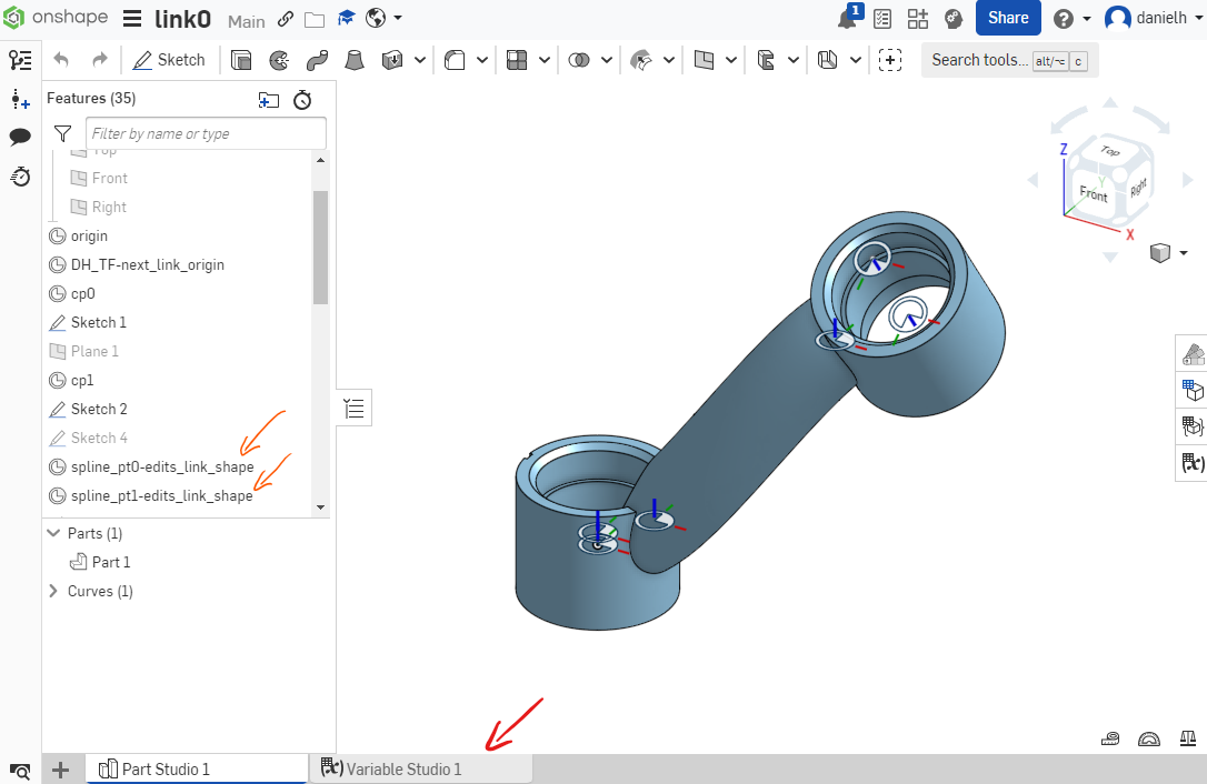
Any link can be edited with newly calculated parameters. Use “Variable Studio 1” tab in the model as show via red arrow in the figure below. It might happen that the link curve is not suitable for the new parameters (it has a unnaturally curved shape or not renders at all). In that case, adjust two curve points by editing their coordinates by double clink on the features “spline_pt0-edits_link_shape” and “spline_pt1-edits_link_shape” as shown via orange arrows in the figure below.

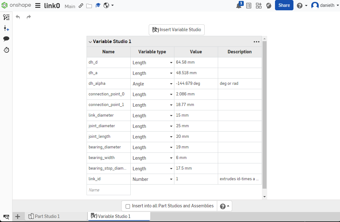
Editing in Variable studio:

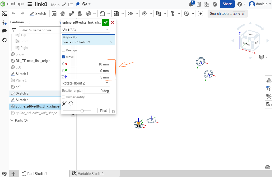
Editing so-called Mate Connectors which determine the shape of the link-curve:

References

[1]

K. Brunnthaler, H.-P. Schröcker, and M. Husty. A new method for the synthesis of Bennett mechanisms. International Workshop on Computational Kinematics, 2005.