Direct (Forward) Kinematics, Inverse Kinematics, and Trajectory Generation

This Jupyter notebook serves as an example of using the package for direct (forward) kinematics, inverse kinematics, and trajectory generation for driving joint. Run it live on Binder platform clicking on the following badge:

Link to the source notebook: https://github.com/hucik14/rational-linkages/blob/main/docs/source/tutorials/trajectory_planning.ipynb

# in case of errors, make sure to have the latest version of the rational-linkages package installed (uncomment the following line and run the cell - it will install the package into your current environment)
# !pip install --upgrade rational-linkages[opt]

# initial import of the required libraries
%matplotlib inline
import numpy as np
import matplotlib.pyplot as plt

from rational_linkages import (RationalMechanism, Plotter, TransfMatrix, MotionInterpolation, PointHomogeneous)

Synthesize Bennett mechanism for given poses.

The poses are given as transformation matrices. They are using European convention - projective coordinates are on first line and translation vector is in the left column.

p0 = TransfMatrix()
p1 = TransfMatrix.from_vectors(approach_z=[-0.0362862, 0.400074, 0.915764],
                               normal_x=[0.988751, -0.118680, 0.0910266],
                               origin=[0.033635718, 0.09436004, 0.03428654])
p2 = TransfMatrix.from_vectors(approach_z=[-0.0463679, -0.445622, 0.894020],
                               normal_x=[0.985161, 0.127655, 0.114724],
                               origin=[-0.052857769, -0.04463076, -0.081766])
poses = [p0, p1, p2]

for pose in poses:
    print('Pose p' + str(poses.index(pose)) + ' as matrix:')
    print(pose)
    print('Pose p' + str(poses.index(pose)) + ' as dual quaternion:')
    print(pose.matrix2dq())
    print('')

Pose p0 as matrix:
[[1., 0., 0., 0.],
 [0., 1., 0., 0.],
 [0., 0., 1., 0.],
 [0., 0., 0., 1.]]
Pose p0 as dual quaternion:
[1. 0. 0. 0. 0. 0. 0. 0.]

Pose p1 as matrix:
[[ 1.          ,  0.          ,  0.          ,  0.          ],
 [ 0.033635718 ,  0.9887513371,  0.1451003257, -0.0362862073],
 [ 0.09436004  , -0.1186800739,  0.9087660701,  0.4000740805],
 [ 0.03428654  ,  0.0910265534, -0.3912673323,  0.9157641843]]
Pose p1 as dual quaternion:
[ 1.         -0.20752242 -0.03338667 -0.06917412 -0.00625114 -0.01412658
 -0.04478577 -0.02637269]

Pose p2 as matrix:
[[ 1.          ,  0.          ,  0.          ,  0.          ],
 [-0.052857769 ,  0.9851611934, -0.1652496366, -0.0463678836],
 [-0.04463076  ,  0.1276549492,  0.886073015 , -0.4456218419],
 [-0.081766    ,  0.1147241778,  0.4330902558,  0.8940196829]]
Pose p2 as dual quaternion:
[ 1.          0.23337393 -0.04278385  0.07779146 -0.00839342  0.02991396
  0.02980046  0.03454444]

Construct curve C(t) from poses and factorize it to obtain Bennett mechanism

c = MotionInterpolation.interpolate(poses)
m = RationalMechanism(c.factorize())

print('C(t):')
for el in m.symbolic:
    print(el)

C(t):
1.0*t**2 - 0.922574886391459*t + 0.225924553870895
0.0527249009995822 - 0.115676757209998*t
-0.000461911731624117*t - 0.00966592244448864
0.0175750001919763 - 0.0385589465872888*t
-0.00189628031924141
0.00675829865504969 - 0.0110435917756025*t
0.00673265674836427 - 0.0203184045107608*t
0.00780443778676431 - 0.0158045843886699*t

Inverse kinematics

theta1 = m.inverse_kinematics(p1)
theta2 = m.inverse_kinematics(p2)
print('Joint angle for pose 1 in rad:', theta1)
print('Joint angle for pose 2 in rad:', theta2)

Joint angle for pose 1 in rad: 0.33082693881455877
Joint angle for pose 2 in rad: 5.892802131407738

Direct (forward) kinematics

pose1_as_dq = m.forward_kinematics(theta1)
pose2_as_dq = m.forward_kinematics(theta2)

pose1_as_matrix = pose1_as_dq.dq2matrix()
pose2_as_matrix = pose2_as_dq.dq2matrix()

print('Pose 1 as matrix:')
print(pose1_as_matrix)
print('Pose 2 as matrix:')
print(pose2_as_matrix)

Pose 1 as matrix:
[[ 1.          0.          0.          0.        ]
 [ 0.03363572  0.98875134  0.14510033 -0.03628621]
 [ 0.09436004 -0.11868007  0.90876607  0.40007408]
 [ 0.03428654  0.09102655 -0.39126733  0.91576418]]
Pose 2 as matrix:
[[ 1.          0.          0.          0.        ]
 [-0.05285777  0.98516119 -0.16524964 -0.04636788]
 [-0.04463076  0.12765495  0.88607302 -0.44562184]
 [-0.081766    0.11472418  0.43309026  0.89401968]]

Simple comparision of input/output matrices

error_pose1 = np.linalg.norm(pose1_as_matrix - p1.array())
error_pose2 = np.linalg.norm(pose2_as_matrix - p2.array())
print('Error in direct kinematics for pose 1:', error_pose1)
print('Error in direct kinematics for pose 2:', error_pose2)

Error in direct kinematics for pose 1: 5.161702277922196e-15
Error in direct kinematics for pose 2: 6.072198263195411e-15

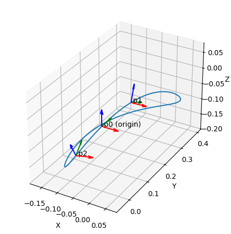
Plot mechanism

p = Plotter(jupyter_notebook=True, steps=500, arrows_length=0.05)
p.plot(m.curve(), interval='closed')
p.plot(p0, label='p0 (origin)')
p.plot(p1, label='p1')
p.plot(p2, label='p2')
p.show()

# if in script mode (not in Jupyter notebook), use the following line to display interactive plot

# p = Plotter(mechanism=m, steps=500, arrows_length=0.05, joint_sliders_lim=0.1)
# p.plot(p0, label='p0 (origin)')
# p.plot(p1, label='p1')
# p.plot(p2, label='p2')
# p.show()

# after calculating the joint angles, the mechanism can be animated using the following code
# p.animate_angles(pos, sleep_time=0.5)

Trajectory generation

total_time_of_motion = 4.  # seconds
frequency = 20  # Hz
num_points = int(total_time_of_motion * frequency)

Joint-space point-to-point trajectory (quintic polynomial scaling)

pos, vel, acc = m.traj_p2p_joint_space(joint_angle_start=theta1,
                                       joint_angle_end=theta2,
                                       time_sec=total_time_of_motion,
                                       num_points=num_points,
                                       generate_csv=False)

%matplotlib inline
plt.figure()
plt.plot(pos)
plt.plot(vel)
plt.plot(acc)
plt.xlabel('Time-step')
plt.ylabel('Joint pos [rad], vel [rad/s], acc [rad/s^2]')
plt.legend(['Pos (origin)', 'Vel (origin)', 'Acc (origin)'])
plt.title('Smooth joint-space trajectory')
plt.grid()
plt.show()

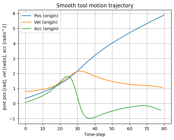
Smooth tool equidistant motion

pos_t, vel_t, acc_t = m.traj_smooth_tool(joint_angle_start=theta1,
                                         joint_angle_end=theta2,
                                         time_sec=total_time_of_motion,
                                         num_points=num_points,
                                         generate_csv=False)

plt.figure()
plt.plot(pos_t)
plt.plot(vel_t)
plt.plot(acc_t)
plt.xlabel('Time-step')
plt.ylabel('Joint pos [rad], vel [rad/s], acc [rad/s^2]')
plt.legend(['Pos (origin)', 'Vel (origin)', 'Acc (origin)'])
plt.title('Smooth tool motion trajectory')
plt.grid()
plt.show()

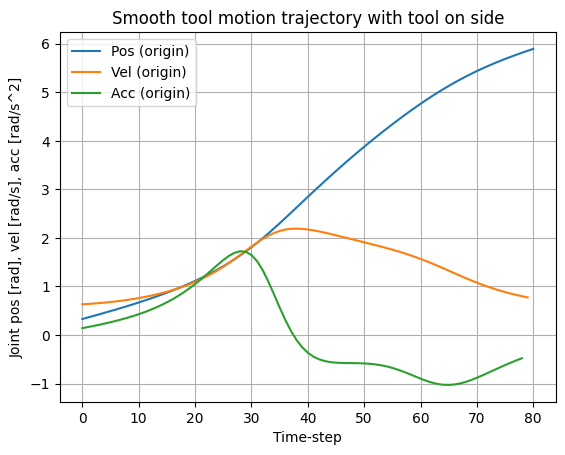
Define a new TCP point that will be taken into account

t_new_tool = PointHomogeneous([1, 0, -0.17, 0])

pos_t2, vel_t2, acc_t2 = m.traj_smooth_tool(joint_angle_start=theta1,
                                            joint_angle_end=theta2,
                                            time_sec=total_time_of_motion,
                                            point_of_interest=t_new_tool,
                                            num_points=num_points,
                                            generate_csv=False)

plt.figure()
plt.plot(pos_t2)
plt.plot(vel_t2)
plt.plot(acc_t2)
plt.xlabel('Time-step')
plt.ylabel('Joint pos [rad], vel [rad/s], acc [rad/s^2]')
plt.legend(['Pos (origin)', 'Vel (origin)', 'Acc (origin)'])
plt.title('Smooth tool motion trajectory with tool on side')
plt.grid()
plt.show()

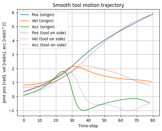
Comparison of all trajectories

plt.figure()
plt.plot(pos_t, 'C0')
plt.plot(vel_t, 'C1')
plt.plot(acc_t, 'C2')
plt.plot(pos_t2, 'C3', linestyle=':')
plt.plot(vel_t2, 'C5', linestyle=':')
plt.plot(acc_t2, 'C4', linestyle=':')
plt.xlabel('Time-step')
plt.ylabel('Joint pos [rad], vel [rad/s], acc [rad/s^2]')
plt.title('Smooth tool motion trajectory')
plt.legend(['Pos (origin)', 'Vel (origin)', 'Acc (origin)',
            'Pos (tool on side)', 'Vel (tool on side)', 'Acc (tool on side)'])
plt.grid()
plt.show()